Inductor: Automated Hypothesis Verification using LLMs and Hierarchical Bayes-like models

Avishek Sen Gupta on 23 June 2025

---

We look at how a Hierarchical Bayes-like model can be used to recursively decompose a hypothesis into sub-hypotheses to form an inference tree. The beliefs of these sub-hypotheses are updated based on the strength of the evidence gathered using MCP tools.

These beliefs are propagated upwards through the inference to indicate the aggregate confidence of the original root hypothesis. This concept is demonstrated in a library called Inductor.

This post has not been written or edited by AI.

Motivation

For the last year or so, I’ve been heavily involved in building reverse engineering tooling dealing with legacy code. This legacy code includes the usual suspects (COBOL, HLASM), but can also include code written in more “modern” stacks, like Java, C#, etc. Much of this tooling is driven through LLMs (isn’t everything these days :-) ?).

However, these efforts have also forced some deeper introspection on my part about how humans deal with comprehending legacy code. There are several studies on models of human comprehension of code (both novices and experts), but for the purposes of this post, I will restrict myself to my own (obviously incomplete) mental model of how I resolve uncertainty when attempting to validate or invalidate a hypothesis.

This could be a hypothesis about anything, for example:

• This routine does not modify this variable.
• This piece of code branches off unconditionally, but does return to the point of origin.
• This memory addresses represents a particular quantity in the domain
• … and so on

Most of the time, we (I?) look for signals which strengthen or weaken my belief in the hypothesis. Some studies call these signals beacons. The result of aggregating all these signals gives me a rough idea of how valid my hypothesis is. It is important to note that this is a sliding scale from “This is definitely false” to “This is definitely true”, and other values like “I’m still not sure” in between.

This seems to be a good fit for Bayesian reasoning. For the purposes of this experiment, I adopted a simple approach which is analogous to using a Hierarchical Bayes Model with a Beta-Bernoulli conjugate for prior-posterior belief calculations (more on that here)

Let’s talk of hypothesis decomposition. Whenever I have a hypothesis, I’m subconsciously breaking it down into smaller hypotheses that I can prove/disprove. Then, I would go and gather evidence for/against these smaller hypotheses, and go back and assess my confidence in my original hypothesis. Essentially, we can think of this as building an inference tree, like so:

The question is: is this something reproducible through LLMs and Bayes-like techniques? This sort of hierarchical modelling is something found in Hierarchical Bayes Models. We will use something similar, but much simpler. We will simply sum up weighted combinations of the evidences for and against the corresponding sub-hypotheses.

I have thus encapsulated some of my learning and experiments into a library called Inductor. I originally meant for it to help me explore inductive logic programming techniques, hence the name (I still might :-) ).

How do we validate a hypothesis?

• Propose a hypothesis (User / LLM)
• Decompose the hypothesis with initial levels of belief (LLM) like so:
  • At every level of decomposition, ask the LLM to decide whether any more decomposition into sub-hypotheses is required. If decomposition is not required, the sub-hypothesis ends with a set of leaf evidence nodes. These are the pieces of evidence that will be gathered to determine the strength of the sub-hypothesis.
• Gather evidence for sub-hypotheses: This is where LLMs can use tools (exposed via MCP tools) to pick the best tool(s) to gather specific pieces of evidence. The LLM decides whether the evidence supports the sub-hypothesis or not.
• Propagate beliefs upward based on summing the (potentially weighted) counts of for/against evidence, all the way up to the original hypothesis (Deterministic)
• The final weighted counts of the for/against evidence at the root provides us a degree of belief in the root hypothesis.

The flow would look something like the following:

In this case, we can simply sum aggregate the counts of the evidences into two buckets:

• Evidence supporting the sub-hypothesis
• Evidence not supporting the sub-hypothesis

Motivating example

As a demonstration, I took a simple HLASM program, ran it through Tape/Z to parse its structure, and exposed its various functionalities to the Langgraph system through an MCP server. Examples of the functionalities exposed were:

• Regex search
• Cyclomatic complexity
• Code in specific sections (labels)
• …etc.

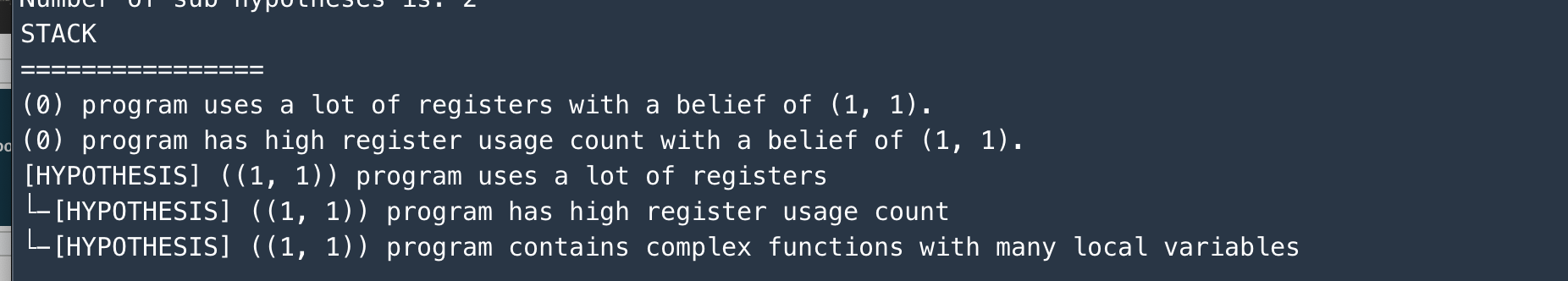
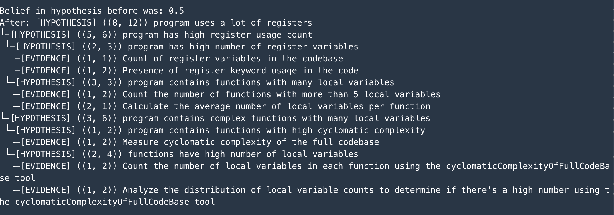
The hypothesis that I asked it to verify was that the program uses a lot of registers. This is shown in the screenshot below.

Beyond this point, the Hypothesis Decomposer component of Inductor starts recursively decomposing this hypothesis into an inference tree, as show by the progression of screenshots below (I intentionally limited the number of branches at each step to 2 for speed of demonstration):

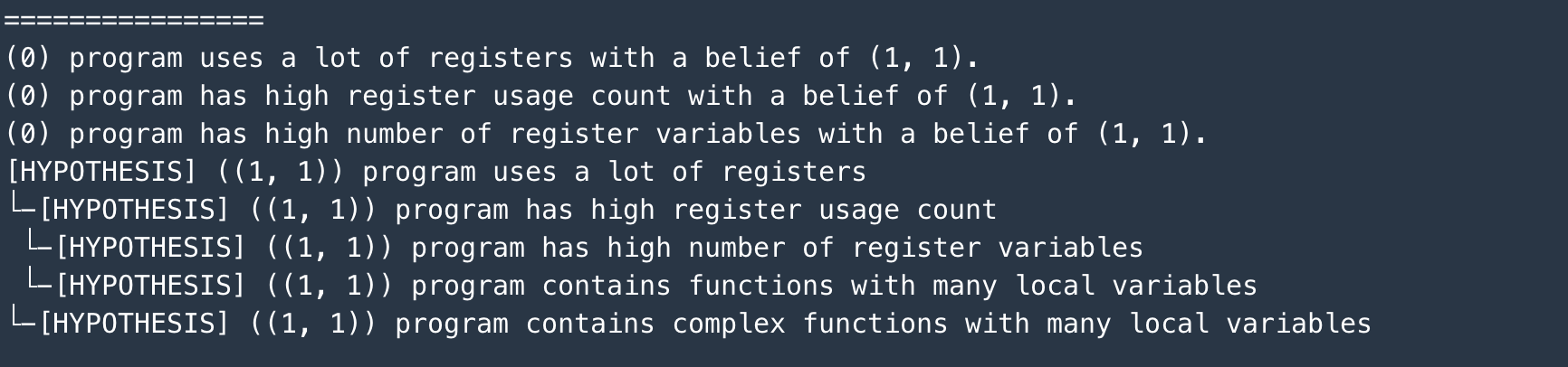
…and so on, until the leaves of evidence are reached.

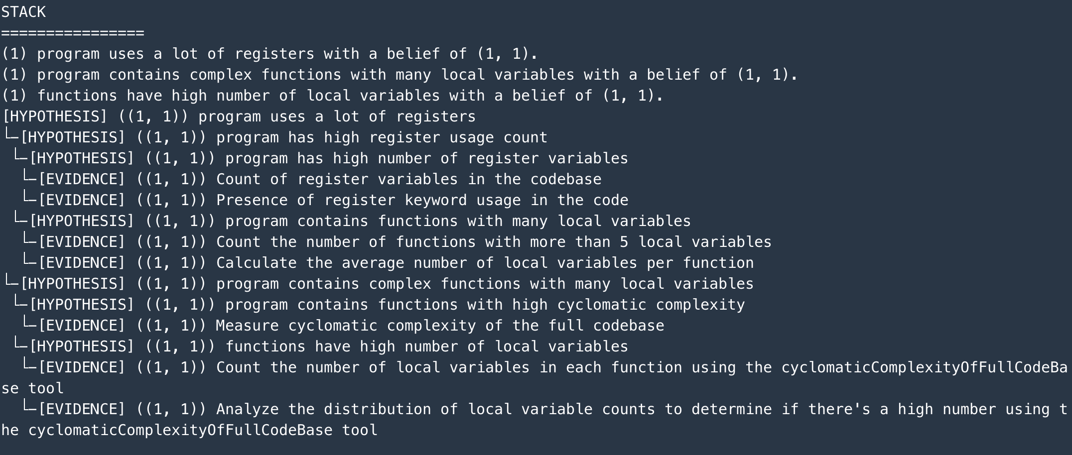
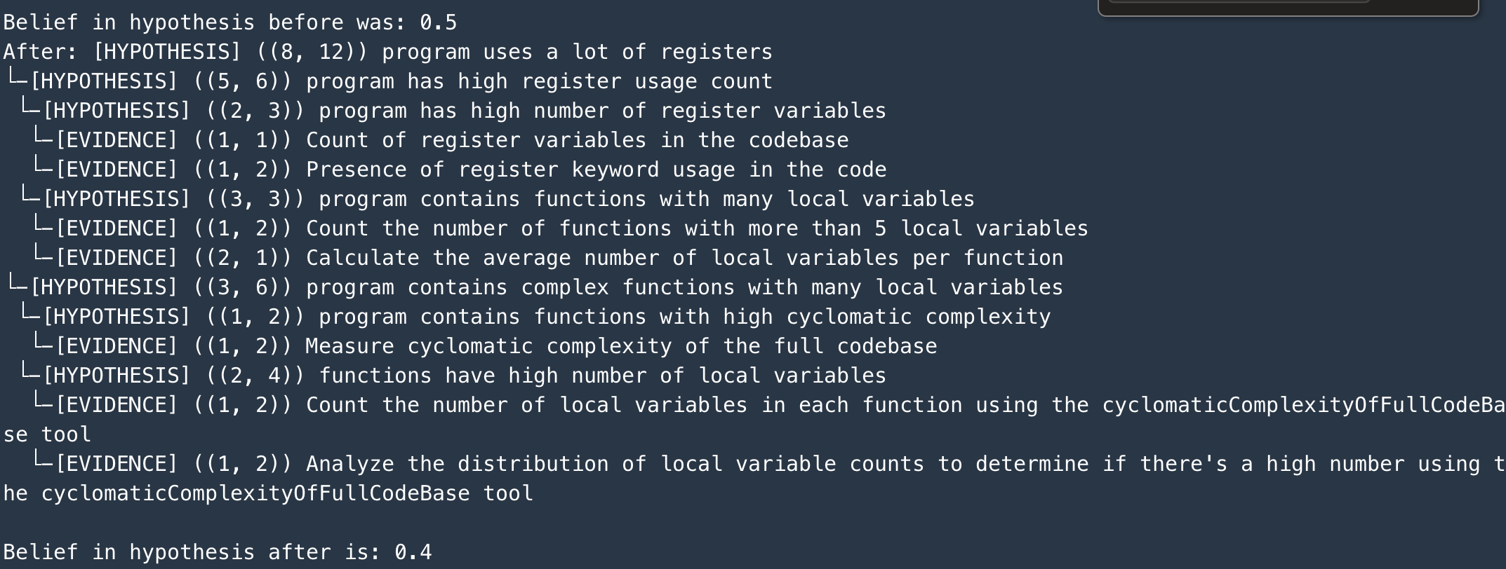
At this point, the inference tree has been built, and the Hypothesis Validator component goes into action, starting to collect evidence, and aggregating the strengths up the hierarchy of the tree. The result is an updated strength of the root hypothesis. As shown in the screenshot below, the original strength was 0.5 (equally likely to be true or false), and the posterior strength came down to 0.4, indicating a weakened belief in the root hypothesis.

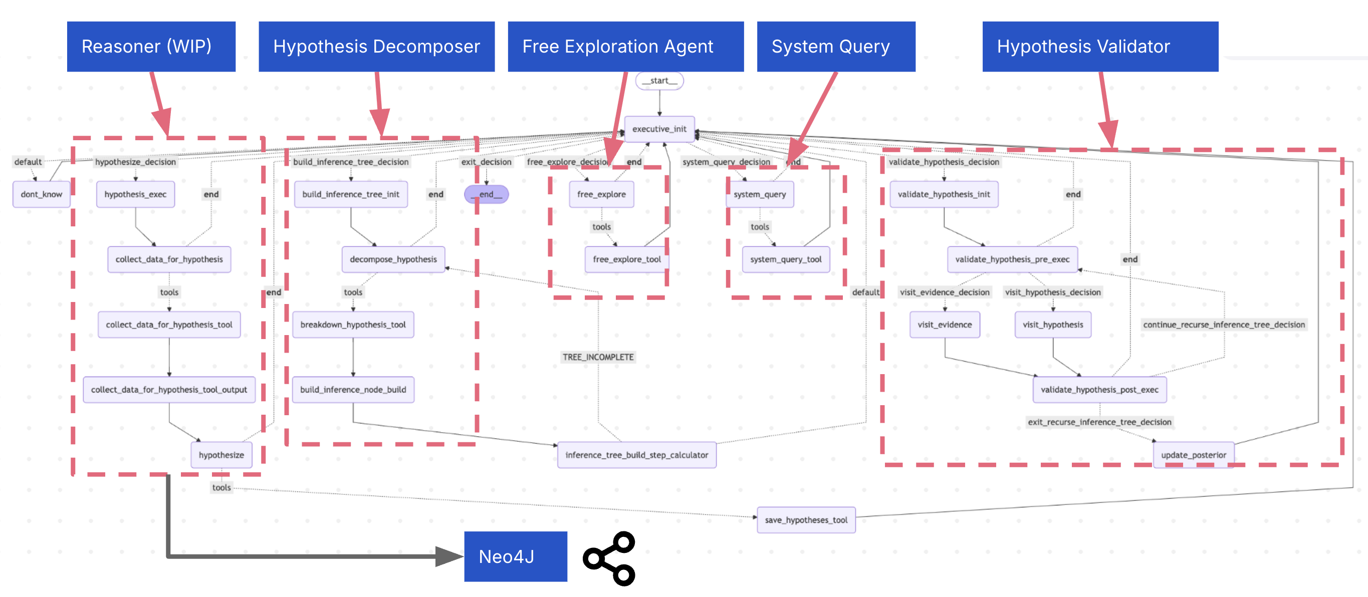
Architecture of Inductor

The overall architecture consists of several parts, some of them more experimental than others at this point. They reflect my early attempts to build a CLI for explore a system for the purposes of reverse engineering using MCP tools. The whole thing is probably meant to be plugged into a larger system. It is essentially a medium-sized Langgraph graph, with the following components:

• Executive Agent: Guides the overall exploration process
• Hypothesis Decomposer: Validates hypotheses through structured inference
• Hypothesis Validator: Explores evidence related to hypotheses and propagates beliefs upwards
• Hypothesizer: Generates hypotheses about code functionality
• Free Explorer: Allows for free exploration of the codebase using MCP tools
• System Query: Answers questions about the MCP tools themselves

Hypothesis Decomposer: Design

The Hypothesis Decomposer component builds the inference tree recursively. There were a couple of options for designing this.

• Build a smaller independent Langgraph graph where each task node corresponds to either aggregation from its child nodes or evidence gathering using MCP tools.
• Build an iterative graph loop and keep track of the recursion state in the agent context. This requires more bookkeeping (like storing current recursion information in a stack), and nodes with dedicated logic to decide when to unroll the recursive call.

In the end, I decided to go with the second option, because it seemed more straightforward; however, I may try out the first approach at some point. The subgraph which implements this component is showb below.

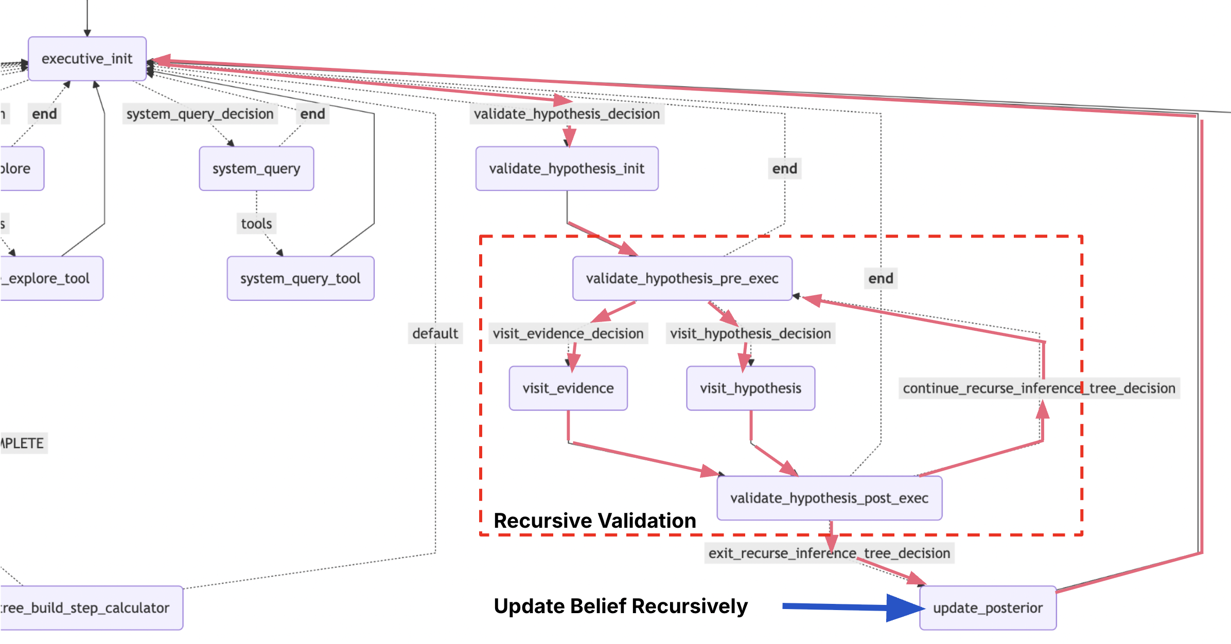
Hypothesis Validator: Design

I followed a very similar approach to the Hypothesis Decomposer component, except this time, we are traversing the inference tree instead of building it. Similar stack-based bookkeeping of the recursion state applies here.

The subgraph which implements this component is showb below.

Caveats and Limitations

• I use the term “belief” pretty loosely. It is intentionally constrained to be between 0 and 1 to reflect a possible Bayesian probability. That more formal interpretation will probably require a more refined modelling. I discuss the analogy briefly in Analogy with Hierarchical Bayes.
• All sub-hypotheses are assumed to be independent of each other. This is often not true. Overlapping, dependent sub-hypotheses need causal connections between them which would normally affect belief propagation.
• The Beta-Bernoulli conjugate-like calculations have been chosen for their simplicity, and aren’t necessarily the best fit to represent the prior and posterior. More sophisticated probability distribution modelling using MCMC, etc. should ideally be done.
• The prompting needs to be more precise to get more contextually correct sub-hypotheses, because the current prompting leads to inferring some sub-hypotheses which make sense in the context of HLASM programs (for example: how would an HLASM program contain complex functions?).

Analogy with Hierarchical Bayes with Beta-Bernoulli conjugate

The above technique is analogous to a Hierarchical Bayes Model where probability distributions are modelled by Beta distributions, and posterior distributions are calculated using the conjugacy of the Beta-Bernoulli pair.

The Beta distribution is a customisable probability distribution, whose shape can be controlled by two parameters \(\alpha\) and \(\beta\). The formula for the distribution is given as:

\[f(x;\alpha,\beta) = k.x^{\alpha-1}.{(1-x)}^{\beta-1}\]

where \(k\) is a constant chosen such that the area under the probability distribution sums to 1. The shapes of the Beta distribution for different values of \(\alpha\) and \(\beta\) are shown below (taken from Wikipedia). As you can see, the shape can vary widely depending upon the parameter combination.

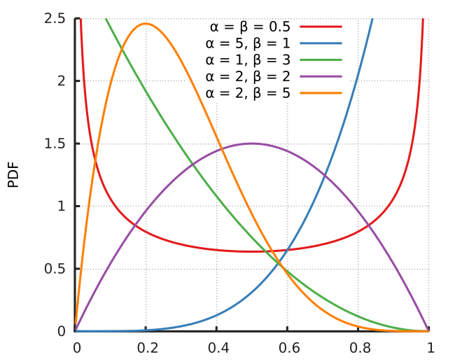
The Beta distribution is frequently used to model experiments with discrete successes/failure counts. If the already observed results are represented by a Beta distribution, then the updated distribution after observing a set of more experiments (successes and failures) can simply be modelled as simple sums of the \(\alpha\) and \(\beta\) parameters. This is analogous to summing up the counts of evidences supporting and not supporting the sub-hypotheses and propagating them up the inference tree.

References

• Inductor
• Tape/Z

---